Review
A logistic regression can be viewed as one neuron NN with linear part and activation part.
Sigmoid function is common function to be used in classification tasks.
The more we stack layer, the more parameters we have. The more our network is able to copy the complexity of our data.
Backpropagation
First we define our cost function.
We want to do batch computation. Since we want to use GPU to compute parallel data together.
\[J(\hat{y},y) = \frac1m\sum^m_{i=1} L^{(i)}(\hat{y},y)
\]
with
\[L^{(i)} = -[y^{(i)}log\hat{y}^{(i)} + (1-y^{(i)})log(1-\hat{y}^{(i )})]
\]
In order to use the chain rule, we need to start with \(w_3,b_3\).
Update:
\[W^{[l]} = W^{[l]} - \alpha\frac{\partial J}{\partial W^{[l]}}
\]
One thing need to notice is that the derivative is linear. If we want to take derivative of J, it is just like taking derivative of L.
With \(a^{[0]} = x\), we have
\[\begin{aligned}
a^{[1]} &=\operatorname{ReLU}\left(W^{[1]} a^{[0]}+b^{[1]}\right) \\
a^{[2]} &=\operatorname{ReLU}\left(W^{[2]} a^{[1]}+b^{[2]}\right) \\
\cdots & \\
a^{[r-1]} &=\operatorname{ReLU}\left(W^{[r-1]} a^{[r-2]}+b^{[r-1]}\right)
\end{aligned}
\]
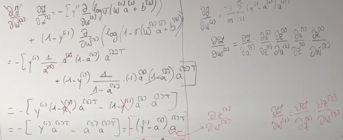
\[\begin{aligned}
&\frac{\partial y}{\partial w^{(3)}}=-\left[y^{(i)} \frac{\partial}{\partial w^{[3]}} \log \sigma\left(w^{[3]} a^{[2]}+b^{[3]}\right)\right) \\
&+\left(1-y^{(i)}\right) \frac{\partial}{\partial w^{(3)}}\left(\log \left(1-\sigma\left(w^{[3)} a^{[2]}+b^{[3]}\right)\right)\right]
\end{aligned}
\]
\[\begin{aligned}
&=-\left[y ^ { ( i ) } \frac { 1 } { a ^ { ( 3 ) } } \cdot a ^ { ( 3 ) } \cdot \left(1-a^{(3)} \cdot a^{(2) T}\right)\right] \\
&\left.+\left(1-y^{(i)}\right) \frac{1}{1-a^{(3)}} \cdot(-1) a^{(3)}\left(1-a^{(3)}\right) \cdot a^{(2)}\right] \\
&=-\left[y^{(i)}\left(1-a^{(3)}\right) a^{(2) T}-(1-y^{(i)}) a^{(3)} \cdot a^{(2) T}\right] \\
&=-\left[y^{(i)} a^{(2) T}-a^{(3)} a^{(2) T}\right]=-\left(y^{(i)}-a^{(3)}) a^{(2)T }\right.
\end{aligned}
\]
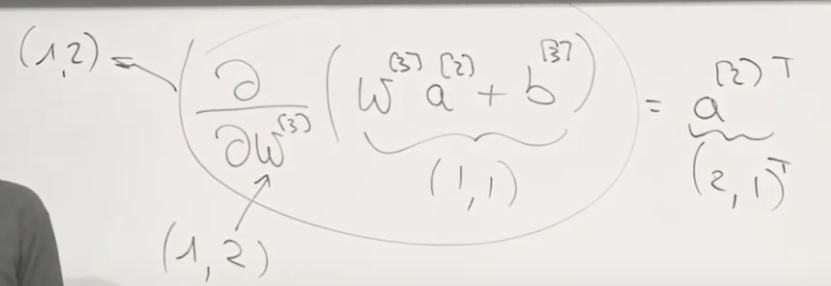
Why we should get \(a^{[2]}\) transposed?
Then we get
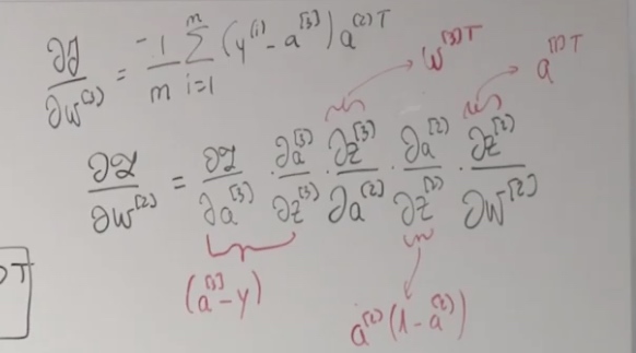
\[\frac{\partial y}{\partial w^{(3)}}=\frac{-1}{m} \sum_{i=1}^{m}\left(y^{(i)}-a^{(3)}\right) a^{(2) T}
\]
Now we are going to send this one into GD.
Then we will use the chain rule to calculate \(\frac{\partial L}{\partial W^{[2]}}\)
\[\frac{\partial L}{\partial w^{(2)}}=\frac{\partial z}{\partial a^{(3)}} \cdot \frac{\partial a^{(3)}}{\partial z^{(3)}} \cdot \frac{\partial z^{(3)}}{\partial a^{(2)}} \cdot \frac{\partial a^{(2)}}{\partial z^{(2)}} \cdot \frac{\partial z^{(2)}}{\partial w^{(2)}}
\]
Where \(z = aw+b\), \(a = \sigma(z)\).
We cannot take derivative on w or b, or we will get stuck.
Since \(a^{[2]T} = \frac{\partial z^{[3]}}{\partial w ^{[3]}}\), also, \(\frac{\partial \mathcal{L}}{\partial w^{(3)}}=\frac{\partial \mathcal{L}}{\partial z^{(3)}} \cdot \frac{\partial z^{[3]}}{\partial w^{(3)}}\)
So, \(\frac{\partial \mathcal{L}}{\partial z^{(3)}} = -(y^{(i)}-a^{[3]})\)
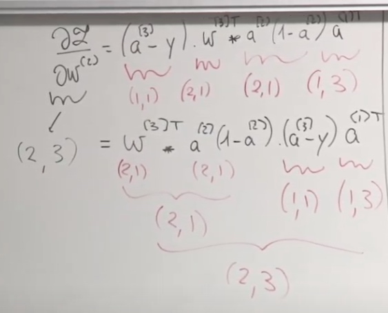
We should also apply the shape analysis.
\[\frac{\partial \mathcal{L}}{\partial w^{(2)}}=\left(a^{(3)}-y\right) \cdot w^{[3] T} * a^{(2)}\left(1-a^{(2)}\right) a^{(1) T}
\]
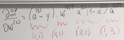
(2,1) and (2,1) do not match together. How could we do on it?
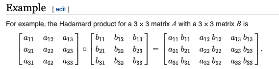
\(w^{[3] T} * a^{(2)}\left(1-a^{(2)}\right) \) is an element-wise product.
For computation efficiency, we need cache.
Improving Your NNs
Activation Functions
- Different Activation Functions
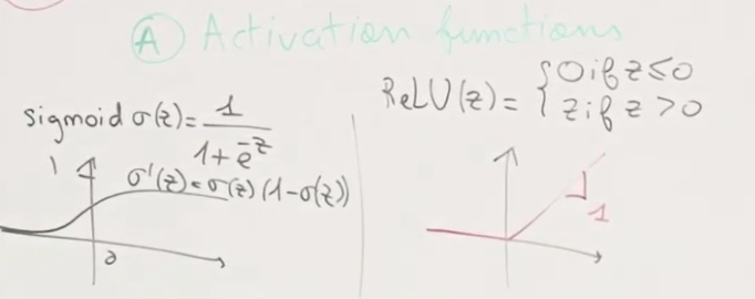
We mainly use sigmoid for classification. When the z becomes really big, our parameters will not going to change during the neurons. So sigmoid works well in linear regioin(middle area), but not in saturating regioins, because the network does not update the parameters properly.
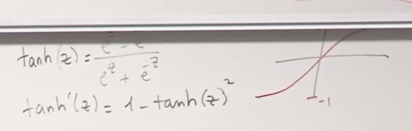
tan is similar to sigmoid.
If we know our results should be between 0 and infinity, then we use ReLu.
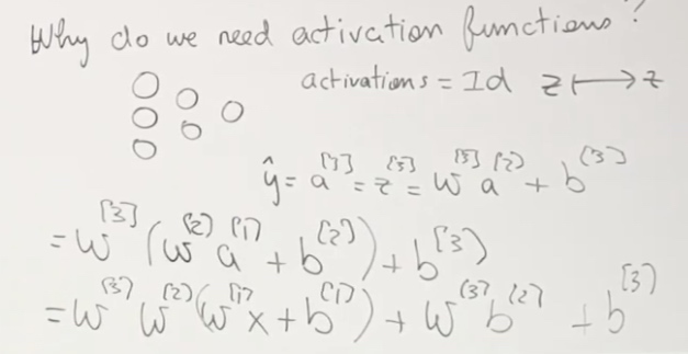
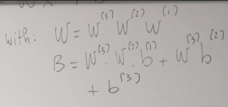
Why do we need activation functions?
If not, things will be like we only have one parameter even if it seems we have several params. No matter how deep is our network.
According to people's experience, we are trying to put one activation function in one layer.
- Initialization/ Normalization
Normalization your input:
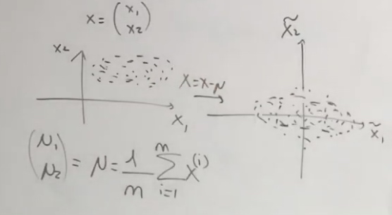
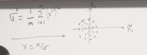
The loss function after and before normalization.
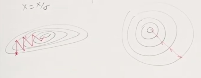
After normalization, gradient descent will go directly to the middle.
One thing to notice is that we need to use mean and standard deviation of training set but not the test set.
Vanishing/Exploding Gradients
Considet a network is very very deep and with only two-dimansional input.
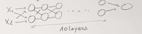 Assume the activation function is identity function and b = 0.
A little bit bigger w will lead to explotion on y.
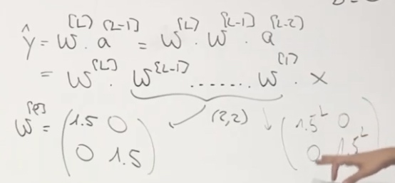
One way to avoid this is initializa the weight properly(close to 1).
Example with 1 neuron:
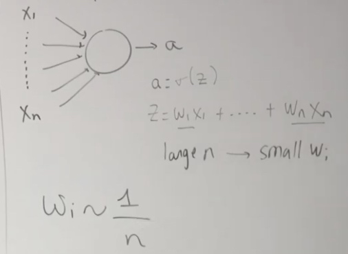
To avoid w exploding, we need to keep wi around 1/n.
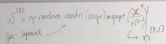
2 for ReLu and 1 for sigmoid.
- Xavien Initialization
- \(W^{{l}}\sim\sqrt{\frac1 {n^{[l-1]}}}\) for tanh
- He Initialization
- \(W^{{l}}\sim\sqrt{\frac2 {n^{[l-1]} + n^{[l]}}}\) for tanh
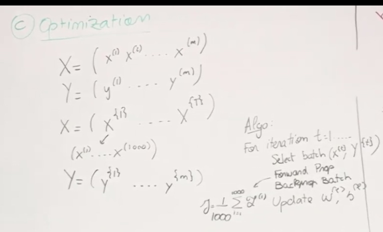
Optimization
batch(vectorization) GD, stochastic GD, mini-batch GD.
Mini batch
m training examples.
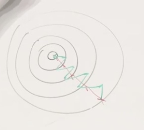
GD + Momentum
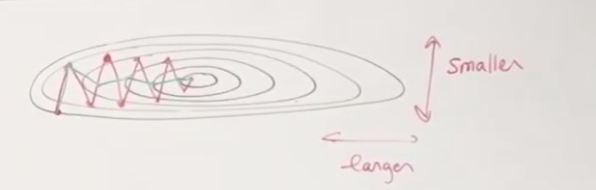
Assume the loss function is very extended in one direction.
It seems we are changing smalled in vertical and larger horizontally.
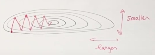
The momentum technique is going to look at past gradients. Look at the past updates you did and try to consider these past updates in order to find the right way to go.
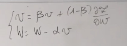
The velocity is going to be the variable that tracks the direction that we should take.